# Load necessary packages using pacman for easier dependency management
pacman::p_load(
  sf,          # For handling shapefiles and geospatial data
  osmdata,     # For fetching OpenStreetMap data
  showtext,    # For adding custom Google fonts
  ggtext,      # For enhanced text formatting in plots
  tidyverse,   # For data manipulation and visualization
  sysfonts,     # For working with system fonts
  glue
)

# Add Google Font
# Add the Posterama 1927 font using its full path
font_add(family = "Posterama", regular = "C:/Users/gonza/AppData/Local/Microsoft/Windows/Fonts/Posterama 1927.ttf")
font_add_google("Roboto Condensed")

# Add local font
font_add("Font Awesome 6 Brands", here::here("fonts/otfs/Font Awesome 6 Brands-Regular-400.otf"))

# Enable custom fonts
showtext_auto()
showtext_opts(dpi = 300)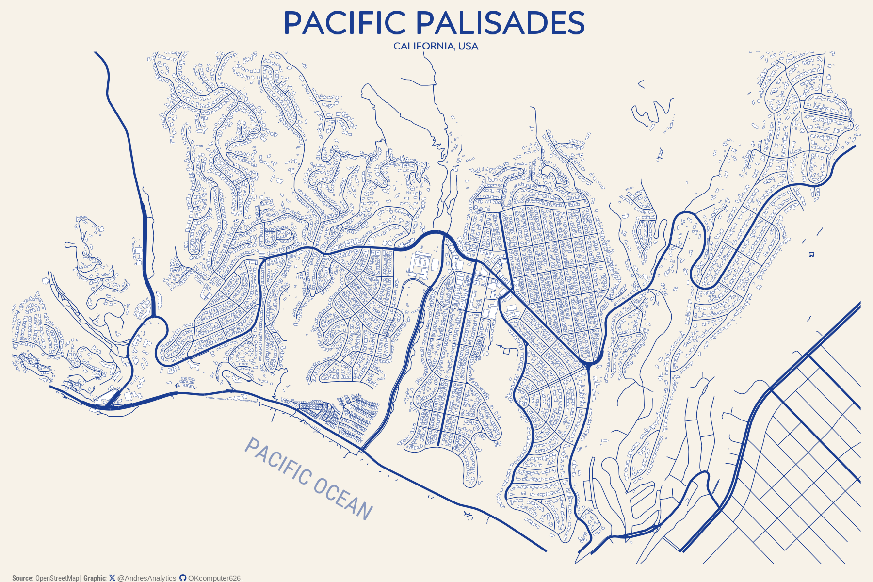
How This Graphic Was Made
1. 📦 Load Packages & Setup
2. 📖 Load Building Footprints
# Load the building footprints from a GeoPackage file
palisades_path <- here::here("Data/Palisades_buildings.gpkg")
buildings <- st_read(palisades_path)
3. 🕵 Filter and Transform PALISADES Data
# Filter for buildings in the PALISADES ZIP Code
palisades <- buildings %>%
  filter(str_detect(SitusZIP, '90272'))

# Reproject PALISADES data to WGS84 (EPSG:4326)
buildings <- st_transform(palisades, crs = 4326)
4. 🤼 Define the Los Angeles Bounding Box
# Define the geographic extent of Los Angeles for the plot
la_bbox <- st_bbox(c(xmin = -118.56, ymin = 34.03, xmax = -118.50, ymax = 34.06), crs = 4326)
la_bb <- st_as_sfc(la_bbox)
5. 🔤 Text
title <- "PACIFIC PALISADES"

subtitle <- "CALIFORNIA, USA"

# Create a social media caption with customized colors and font for consistency in visualization
social <- andresutils::social_caption(font_family = "Roboto Condensed", icon_color = "#1A3D91", font_color = "grey45")

# Construct the final plot caption by combining TidyTuesday details, data source, and the social caption
cap <- paste0(
  "**Source**: OpenStreetMap | **Graphic**: ", social
)
6. 🗺️ Download OpenStreetMap Data
# Fetch major streets
la_big <- la_bb %>%
  opq() %>%
  add_osm_feature(key = "highway",
                  value = c("motorway", "primary", "secondary", "tertiary", "trunk")) %>%
  osmdata_sf()

# Fetch street connectors (links)
la_links <- la_bb %>%
  opq() %>%
  add_osm_feature(key = "highway",
                  value = c("motorway_link", "primary_link", "secondary_link",
                            "tertiary_link", "trunk_link")) %>%
  osmdata_sf()

# Fetch minor streets
la_small <- la_bb %>%
  opq() %>%
  add_osm_feature(key = "highway",
                  value = c("residential", "road", "footway")) %>%
  osmdata_sf()
7. 📊 Plot
# Plot the streets and building footprints
p <- ggplot() +
  geom_sf(data = la_big$osm_lines, inherit.aes = FALSE, color = "#1A3D91", linewidth = 0.5) +
  geom_sf(data = la_links$osm_lines, inherit.aes = FALSE, color = "#1A3D91", linewidth = 0.25) +
  geom_sf(data = la_small$osm_lines, inherit.aes = FALSE, color = "#1A3D91", linewidth = 0.15) +
  geom_sf(data = palisades, fill = "#FFFFFF", color = "#1A3D91", linewidth = 0.05) +
  annotate("text", x = -118.54, y = 34.034, label = "PACIFIC OCEAN", family = "Roboto Condensed", angle = -30, color = "#1A3D91", alpha = 0.5) +
  coord_sf(xlim = c(-118.56, -118.50), ylim = c(34.03, 34.06)) +
  theme_void() +
  theme(
    text = element_text(family = "Posterama"),
    plot.title = element_markdown(color = "#1A3D91", hjust = 0.5, size = 16, face = "bold"),
    plot.subtitle = element_markdown(color = "#1A3D91", hjust = 0.5, size = 5, margin = margin(t = 1)),
    plot.caption = element_markdown(family = "Roboto Condensed", hjust = 0, size = 3.5, color = "grey45"),
    panel.background = element_rect(color = NA, fill = "#F7F2E8"),
    plot.background = element_rect(color = NA, fill = "#F7F2E8")
  ) +
  labs(
    title = title,
    subtitle = subtitle,
    caption = cap
  )
8. 💾 Save
# Save the plot as a high-resolution PNG file
ggsave("Palisades Map.png", p, height = 4, width = 6)
9. 🚀 GitHub Repository
TipExpand for GitHub Repo
Explore the complete code for this visualization in the following Quarto file: Palisades Map.qmd.
For additional visualizations and projects, click here.
Citation
For attribution, please cite this work as:
Gonzalez, Andres. 2025. “Pacific Palisades.” January 15,
2025. https://andresgonzalezstats.com/visualization/Visualizations/2025/LA
Wildfire/Palisades Map.html.